Feedback Trading and the Chinese Put Warrants Bubble

Neil D. Pearson, Zhishu Yang, Qi Zhang
Jul 27, 2022

There was a bubble in the prices of put warrants traded on the Shanghai and Shenzhen stock exchanges during the summer of 2007. We use investor trading records from a large securities firm to show that put warrant investors engaged in a particular form of feedback trading. This feedback trading exacerbated an initial run-up in put warrant prices caused by a change in the stock transaction tax, and created the bubble.

The term “financial bubble” frequently appears in the media, industry reports, and discussions of regulatory policies. For example, the 1996–2000 run-up in the prices of US technology stocks, and the dramatic increases in Chinese stock prices that began in 2014 and continued through June 2015, are often referred to as bubbles. Such apparent bubbles interest academic researchers because they challenge the widespread view that financial market prices should be closely connected to rational expectations of securities’ future cash flows. The economic mechanisms that drive financial bubbles are also likely to exist during non-bubble periods. Thus, studying bubbles can shed light on the factors that determine securities prices during all periods.

There are two leading theories to explain bubbles. The first is the resale option theory proposed by Scheinkman and Xiong (2003), which states that investors are willing to pay a price that exceeds their estimate of a security’s fundamental value, because they have a “resale option” to sell the security if their belief changes and other investors become more optimistic and have an estimate of fundamental value that exceeds their own. Securities are held by the investors with the highest estimates of fundamental value, but market prices exceed investors’ estimate of fundamental value because each security’s market price includes the value of the resale option.

The second theory involves extrapolative beliefs, as, for example, in Barberis et al. (2018), which states that investors’ beliefs about future price changes are partly based on extrapolating past price changes, so the investors anticipate that a rising trend will continue. Because an exogenous shock to a security’s fundamental value will cause a security’s price to rise, a large exogenous shock can create a bubble, as investors with extrapolative beliefs will expect the value to continue to rise and therefore be willing to pay a price that exceeds the fundamental value. Shiller (2015) describes a similar mechanism in which a precipitating event causes an asset price to rise, buying by extrapolating investors causes further price increases, and social contagion attracts new investors whose buying also contributes to the bubble.

Both theories are appealing. But do they capture the key features of investor trading during bubbles? One challenge to the empirical analysis of bubbles is that there is often disagreement about whether a particular episode was a bubble. For example, while some scholars take it for granted that the 1996–2000 run-up in the prices of US technology stocks was a bubble (e.g., Brunnermeier and Nagel 2004), Pástor and Veronesi (2006) and Li and Xue (2009) suggest that the price movements may have been consistent with rational revisions of beliefs about future growth opportunities and uncertainty.

In Pearson, Yang, and Zhang (2021), we take advantage of Xiong and Yu’s (2011) analysis showing that there was a bubble in the prices of Chinese put warrants during the summer of 2007. Each put warrant gave the investor the right to sell stock for a fixed price known as the strike price. A warrant’s maximum payoff would occur if the stock price was zero on the date the warrant expired. In this case the holder of the put warrant could deliver a worthless stock and receive the strike price; the net payoff to the investor would be the strike price. Because the maximum payoff is the strike price, prior to expiration the warrant value must be less than or equal to the strike price. In addition, when the stock price is very high it is almost certain that a put warrant will eventually expire worthless, and the current value must therefore be close to zero. Xiong and Yu (2011) show that the puts traded actively at non-zero prices when their values were almost certainly close to zero. In addition, at times some of the puts traded at market prices greater than their strike prices, which should be impossible and cannot be reconciled with any rational model.

We use investor trading records from a large Chinese securities firm to investigate the factors that created the put warrants bubble. We discover that investors’ trading decisions depended on their past realized returns from trading put warrants, that is, we identify a particular form of feedback trading. We also identify a precipitating event that caused a large initial rise in prices, and show how the feedback trading interacted with the initial increase in prices to create the bubble.

The event that started the bubble was a tripling of the transaction tax on stock trading, which was announced at midnight on May 30, 2007, and took effect immediately at the opening of trading on May 30. The tax change was a regulatory reaction to the apparent overvaluation of the Chinese stock markets and led to immediate one-day declines of 6.15% and 5.78% in the Shanghai and Shenzhen stock indexes. These declines may have drawn attention to the put warrants, because, due to the prohibition on short sales of stock then in effect, put warrants were the only instruments with payoffs that were decreasing in stock prices. The increase in the transaction tax also made warrant trading more desirable for short-term speculative investors, as warrants were exempt from the tax.

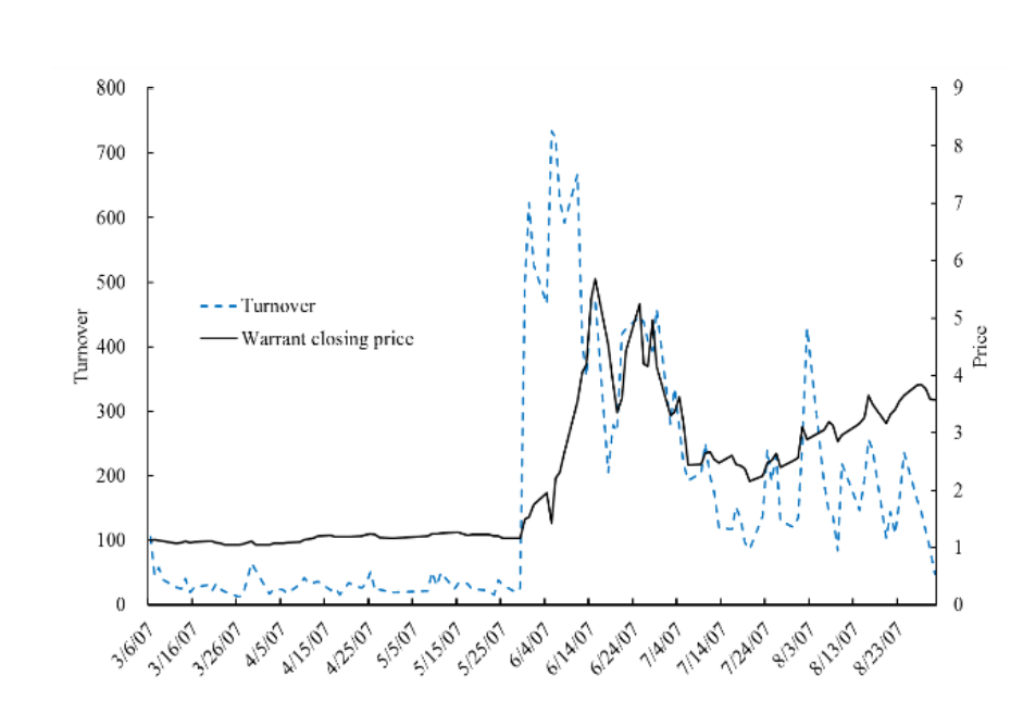
Using the Hualing put warrant as an example, Figure 1 shows the turnover and prices during a six-month period centered on May 30, 2007. The figure shows that turnover increased remarkably on May 30it was 19 times the turnover on May 29. On average, the put warrants that were trading on May 30 experienced a 12-fold increase in turnover. Accompanying the increase in turnover, warrant prices also rose sharply. The Hualing put warrant price increased from 1.16 on May 29 to 1.49 on May 30, for a return of 28%. The average one-day return of the warrants trading on May 30 was 57.6%. The figure also shows that the price of the Hualing put warrant continued to rise after May 30, 2007. This further increase in the price was due to feedback trading, which we discuss next.

Figure 1: Price and turnover of the Hualing put warrant

Daily closing price (solid black line, right-hand axis) and turnover (dotted blue line, left-hand axis) of the Hualing put warrant in March–August 2007, a six-month window approximately centered on May 30, 2007. The figure shows that turnover jumped sharply on May 30 and the price rose sharply on and shortly after that date. This figure was originally published as Figure 1A in Pearson, Yang, and Zhang (2021).

Using hazard rate regressions, we show that investors whose previous warrant trades were profitable were likely to buy warrants again. This is a form of feedback trading, though based on the investors’ own returns rather than publicly observed market prices. The positive feedback trading existed throughout the warrants’ lives, not just during the bubble. It was important starting on May 30, 2007, because the large return on that date caused many investors’ trades to be profitable, leading to additional buying and further positive returns.

We estimate investors’ buying due to feedback trading as follows. For each warrant, investor, and date, we use the hazard rate regressions to compute the probability that the investor will buy on the next trading date. We then estimate the investor’s trade size as their past average trade size. Combining the probability and the estimate of trade size, we have, for each warrant, investor, and date, an estimate of the expected trading volume on the next trade date. We then compute a second estimate of expected trading volume assuming that the investor’s trading does not depend on past returns, that is, using the hazard model but setting the coefficients on past returns equal to zero. The difference between the two estimates is the expected trading volume due to feedback trading for a particular warrant, investor, and date. Aggregating across investors, and then scaling up to the whole market using the reciprocal of the share of market-wide put warrant volume traded by the securities firm’s customers, we obtain an estimate of buying due to feedback trading for each warrant and date.

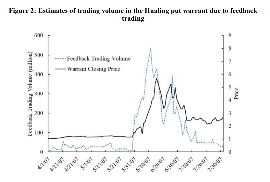
Again using the Hualing put warrant as an example, Figure 2 plots our estimates of buying due to feedback trading in April–July 2007, along with the daily warrant closing price. The results are similar for the other warrants that were trading on May 30, 2007. There was relatively little feedback trading prior to May 30, because warrant prices displayed little variation before that date. Then the initial increase in prices on May 30 created a jump in feedback trading, which caused an additional increase in prices, exciting more feedback trading, and further price increases. The two series displayed in the figure are remarkably similar, consistent with the hypothesis that feedback trading drove the bubble.

Estimates of trading volume due to feedback trading for the Hualing put warrant are shown for April–July 2007, a four-month window approximately centered on May 30, 2007. The figure displays the total estimated feedback trading volume of investors who previously completed at least one warrant trade (dashed blue line, left-hand axis) and the warrant daily closing price (solid black line, right-hand axis). This figure was originally published as Figure 4A in Pearson, Yang, and Zhang (2021).

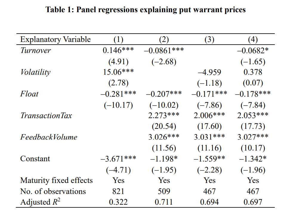
We use panel regressions to provide additional evidence that the combination of the tax change and feedback trading explains the bubble. In their analysis of the bubble, Xiong and Yu (2011) consider a “zero fundamental period” in which the fundamental values of the put warrants were close to zero to ensure that their results are not confounded by variation in the warrants’ fundamental values. They regress warrant prices on turnover, estimates of the warrants’ return volatilities, and the warrants’ float. They obtain significantly positive coefficients on turnover and volatility, which they interpret as consistent with the resale option theory. The results of this regression specification are shown in column 1 of Table 1.

Results of panel regressions explaining put warrant prices during the zero-fundamental period defined by Xiong and Yu (2011). Turnover is market trading volume divided by the number of outstanding warrants, and then divided by 100; Volatility is computed from intraday five-minute returns and then annualized; Float is the daily total number of warrants outstanding, in billions; TransactionTax equals one if the date is May 30, 2007, or later; and FeedbackVolume is the estimate of buying due to feedback trading computed from stratified hazard rate regressions that model investors’ purchases of put warrants. Column 1 replicates some of the results in Xiong and Yu’s (2011) Table 5. Columns 2, 3, and 4 add the estimates of feedback volume and the transaction tax indicator variable to the specifications. All specifications include maturity fixed effects. t-statistics (in parentheses) are based on standard errors clustered by date to account for heteroscedasticity and correlation within a trading day. The results in this table were originally reported in Tables 6 and 8 of Pearson, Yang, and Zhang (2021).

But if feedback trading explains the put warrants bubble, then we expect it, rather than trading volume and volatility, to explain the level of put warrant prices during the bubble period. We explore this hypothesis by augmenting the Xiong and Yu (2011) regression specifications to include both our estimates of feedback trading volume and an indicator variable that equal one for dates on and after May 30, 2007, as additional covariates. The results of specifications that include these additional covariates are displayed in columns 2, 3, and 4 of Table 1. They show that the estimates of feedback volume explain put warrant prices during the zero fundamental period. Once we include the additional covariates turnover and volatility are no longer significantly positively related to put warrant prices. Similar panel regressions, the results of which are not reported here, show that the first differences of our estimates of feedback trading volume explain put warrant returns.

Our results lend support to extrapolative theories, for example, Barberis et al. (2018), as they provide evidence that a form of feedback trading explains the put warrants bubble. While our results for the Chinese put warrants bubble do not lend support to the resale option theory, that theory may play an important role in other bubbles.

References

Barberis, Nicholas, Robin Greenwood, Lawrence Jin, and Andrei Shleifer. 2018. “Extrapolation and Bubbles.” Journal of Financial Economics 129 (2): 203–27. https://doi.org/10.1016/j.jfineco.2018.04.007.

Brunnermeier, Markus K., and Stefan Nagel. 2004. “Hedge Funds and the Technology Bubble.” Journal of Finance 59 (5): 2013-40. https://doi.org/10.1111/j.1540-6261.2004.00690.x.

Garber, Peter M. 1989. “Tulipmania.” Journal of Political Economy 97 (3): 535-60. https://doi.org/10.1086/261615.

Li, C. Wei, and Hui Xue. 2009. “A Bayesian’s Bubble.” Journal of Finance 64 96): 2665-2701. https://doi.org/10.1111/j.1540-6261.2009.01514.x.

Pástor, Ľuboš, and Pietro Veronesi. 2006. “Was There a NASDAQ Bubble in the Late 1990s?” Journal of Financial Economics 81 (1): 61–100. https://doi.org/10.1016/j.jfineco.2005.05.009.

Pearson, Neil D., Zhishu Yang, and Qi Zhang. 2021. “The Chinese Warrants Bubble: Evidence from Brokerage Account Records.” Review of Financial Studies 34:264–312. https://doi.org/10.1093/rfs/hhaa037.

Scheinkman, José A., and Wei Xiong. 2003. “Overconfidence and Speculative Bubbles.” Journal of Political Economy 111 (6): 1183-1220. https://doi.org/10.1086/378531.

Shiller, Robert J. 2015. Irrational Exuberance. Princeton, NJ: Princeton University Press.

Xiong, Wei, and Jialin Yu. 2011. “The Chinese Warrants Bubble.” American Economic Review 101 (6): 2723-53. https://doi.org/10.1257/aer.101.6.2723

Tags: Warrants Bubble , Feedback Trading , Securities Firm , Warrant Trades

Feedback Trading and the Chinese Put Warrants Bubble

Latest

Most Popular